In this post, we will explore the concept of simulating real-world processes using a toy problem commonly encountered in logistics planning.
Problem Statement
The officials of a city are interested in gaining a better understanding of their emergency response services. They want to determine if the response times in the city are below a certain threshold and identify any potential bottlenecks that can be addressed.
Approach: Simulation
Simulating the data provides a practical way to analyze and address the problem at hand. Simulation involves the imitation of real-world processes over time. However, it is essential to explicitly state the assumptions made during the simulation. Failing to do so can lead to inaccurate results.
To illustrate this, let’s consider an example involving modeling the heights of a population. Since height is a continuous measure and people generally do not deviate significantly from the average, the Normal Distribution is an appropriate choice. The Normal Distribution is motivated by the fact that most of the density is concentrated around the mean, as demonstrated by the 68-95-99 rule.
Using a different distribution, such as the Binomial Distribution, to model height would be similar to approximating cows as spheres or cubes in high school physics. While it may work to some extent, it lacks the elegance and accuracy of the Normal Distribution.
Tangent: If you’re interested in understanding why this approximation would have worked, I recommend reading about the Central Limit Theorem.
Step 1: Generate a sample dataset
We need to generate data. But what data specifically? First of we need a way to generate \(n\) points on a 2D grid.
1
2
3
4
5
6
7
8
9
10
11
12
13
14
15
16
17
18
19
20
21
22
23
24
25
26
27
28
29
30
31
32
33
34
def random_coords(n=5, bounds=(50.770, 50.859, 4.248, 4.496)):
    """
        Generates random uniform points on a plane
    """
    # Brussels bounds
    # 50.770883, 4.361551 - south
    # 50.928138, 4.363065 - north
    # 50.863287, 4.248941 - east
    # 50.859386, 4.496820 - west
    x = np.random.uniform(bounds[0], bounds[1], n)
    y = np.random.uniform(bounds[2], bounds[3], n)

    for i in range(n):
        yield x[i], y[i]

def gen_correlated_points(x_prime, y_prime, n=2):
    """
        Given a coordinate (x', y') generate 2D points around it
        with a random covariance.
    """
    A = np.random.uniform(0.05, 0.15, (2, 2))
    cov = np.dot(A, A.transpose())

    cov = cov*np.random.uniform(-0.2, 0.2)

    p1 = np.random.multivariate_normal([x_prime, y_prime], cov, size=n)

    # how many people need to be transported/assisted
    pos = np.random.poisson(lam=1, size=(n, 1.3))
    pos[pos == 0] = 1  # at least 1
    np.random.shuffle(pos)
    data = np.hstack((p1, pos))

    return data
There are 2 functions here that will help us achieve our goal.
random_cords-> takes in \(n\) and a bounding region (for a city, but its not necessary it just looks good on a map)gen_correlated_points-> takes in a point \((x_{prime}, y_{prime})\) and generates a correlated blob of points with a random covariance matrix.
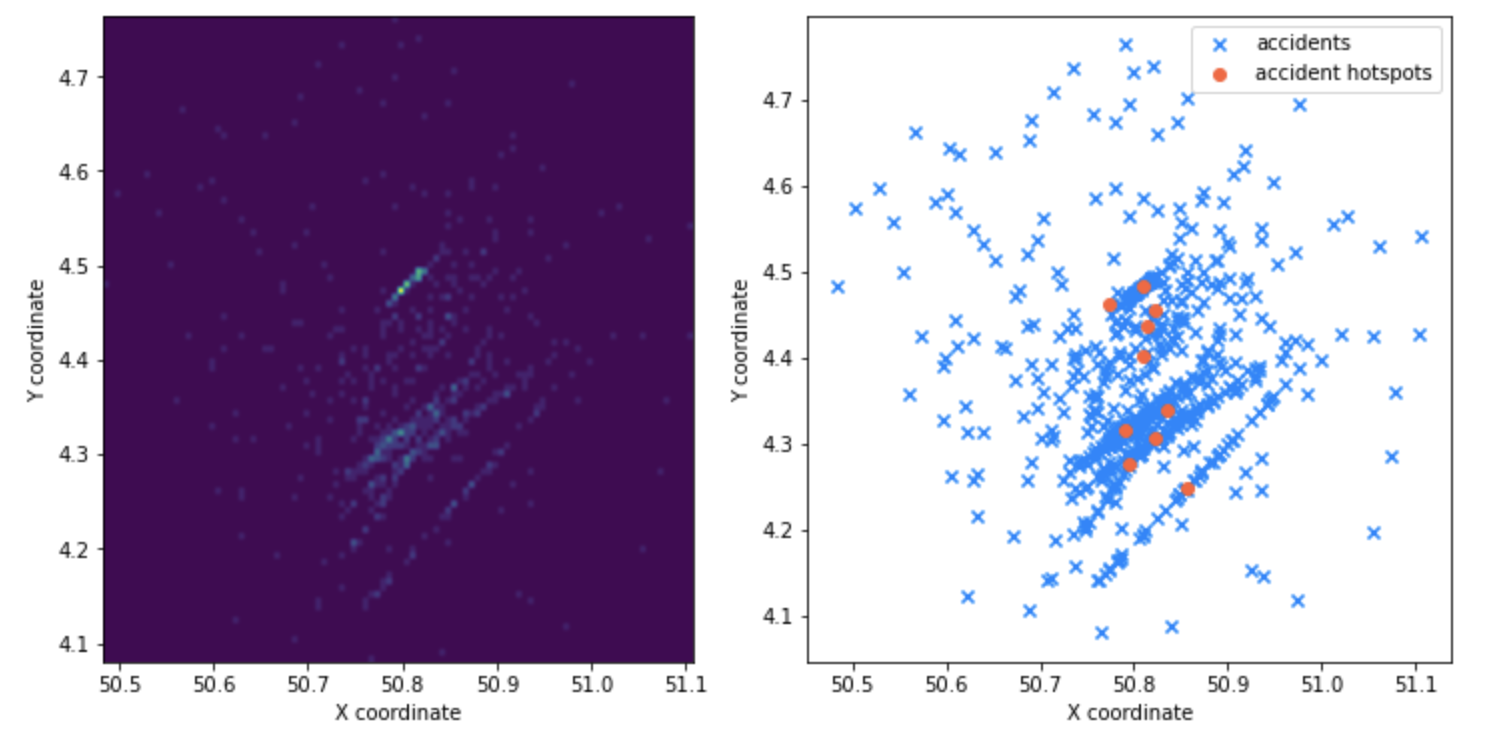
Tha base idea here is that we need a way to generate random points on a grid, then a way to generate a set of correlated points. What this mimics is the ability of bad neighborhoods or roads where a lot of emergency services are needed.
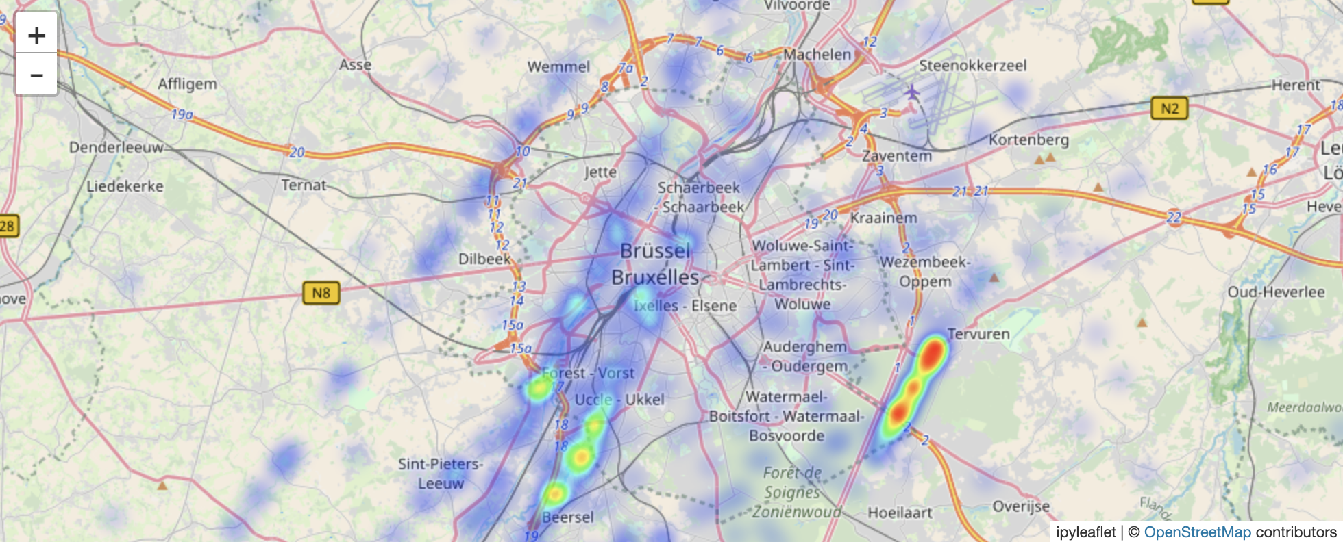
Or looking it through a bit more abstractly, a heatmap and a scatter-plot tells us the proximity of these points.
Step 2: Repeat multiple times?
We cannot create one dataset, analyze it and hope that the public will trust our analysis. We need to generate a lot of these
datasets and perform analysis on top of them, so to say that we ensure the public of our work. We can go about and generate using
the same algorithm we devised in the first section. However, this would mean a lot of parameter tunning, and generally annoying to
parametrize correctly. We will go about and replicate the gist of our dataset using GMM (Gaussian Mixture Models).
scikit-learn has an implementation of GMM and it is simple to use.
1
2
3
4
5
6
7
8
9
from sklearn.mixture import GaussianMixture as GMM

gmm_models = []

for n in range(1, 20, 2):
    gmm = GMM(n_components=n, covariance_type='full', n_init=20, warm_start=True)
    gmm_fitted = gmm.fit(data)
    labels = gmm_fitted.predict(data)
    gmm_models.append((gmm_fitted, labels, gmm_fitted.bic(data)))
Note: We generate a lot of these mixture models to try and understand how many “clusters” of points are there, and use BIC score to select the best one fitting our previously generated data.
Another interesting thing about GMM is that they are just a bunch of gaussian distributions. We can sample as many points as we want, and we are not bound by any parameter to generate a new sample.
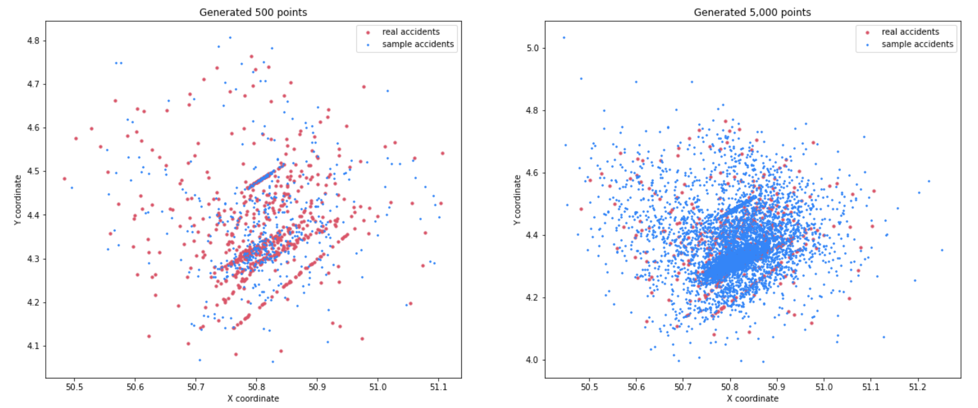
This works well for small number of points (which is our goal), however, we if we sample more we can see the gaussians clusters which are not that “ideal.”
Step 3: Analysis
Now we have come to the interesting part of this post. First we need a couple of emergency care centers like hospitals, but this analysis is similar for other emergency vehicles like police or fire department. We can use the functions from step one to create some uniform points on the map that represent the hospitals.
The number of hospitals in a city is relatively small (5-10) in medium cities, and each hospital has their fleet of emergency vehicles. The latter is needed due to the logic we will implement will include the availability of a their vehicles to respond to an emergency. Note: these are assumptions that are needed to drive forward the simulation.
The logic of our simulation is fairly easy, we have \(m\) hospitals and \(n\) accidents we need to attend to. Each hospital \(m_i\) has \(x\) vehicles at their disposal. Given an accident event \(e\) we will assign the first responder based on two criteria:
- Closest hospital
- Has the availability at that point in time (otherwise add a \(\epsilon \sim N(20, 5)\) to the delay)
1
2
3
4
5
6
7
8
9
10
11
12
13
14
15
16
17
18
19
20
21
22
23
24
def logic(xy_acc, amb_val, availability):
    distances, indices = nbrs.kneighbors(xy_acc)
    distances *= 50 # since cords are gps points, just a trick to get "human" distances

    avg_speed_amb = np.random.normal(60, 5, size=len(centers))
    epsilon = np.random.normal(20, 5, size=len(xy_acc))

    tta_s = []
    for i in range(len(xy_acc)):
        not_found = True
        for j in range(len(centers)):
            if availability[ indices[i][j] ] >= amb_val[i]:
                tta = (distances[i][j] / avg_speed_amb[j])*60
                tta_s.append(tta)

                # assign
                availability[indices[i][j]] -= amb_val[i]
                not_found = False
                break

        if not_found:
            tta_s.append(epsilon[i])

    return np.array(tta_s)
The code above has a lot of assumptions that do not reflect the real-world, but sometimes we just need some spherical cows to make our job a bit easier.
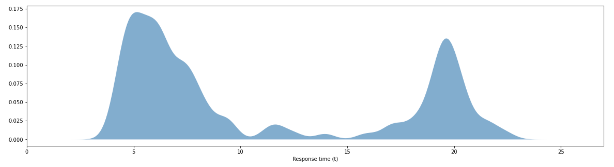
The resulting diagram is the response time given 50 iteration with the logic we described. We can see that most of the density of this KDE is clustered near 2.5 minutes to 10 minute response. However, we see a spike at 20 minute response time, this is the effect of \(\epsilon\) that we drew whenever all hospitals had their vehicles associated with other events. This is the worst case part. One way to control this from not happening is have more emergency vehicles at your disposal. However, by how much is a post for another day and another time.
Conclusions
In this post we have seen how to generate data given a toy problem. The data we generated does not mimic the real world by no means, however, this is good enough for us to dive into some kind of analysis. As we saw in our case, the goal was to get an average time to serve each event, given our assumptions. In the real-world you would not need to generate data for this problem, as the data will be given. However, having the knowledge to create a sample dataset for yourself, can make your workflow faster and understand the variables involved better.
Try to have fun with a toy problem from time to time!