There exists a empirical law in statistics called Benford’s Law. It is so ubiquitous that it shows up in all kind of strange places. Before diving deeper into this topic, let me as you a question: What is the occurrence rate of the leading digit in a dataset representing populations of various countries? You would expect to be uniform, there shouldn’t be a difference between countries that start with 2 (be that thousands, up to millions), between countries that have a leading digit of 8. From personal experience, you would count some popular countries that validate your assumption. However, that is not the truth. As shown in figure 1.
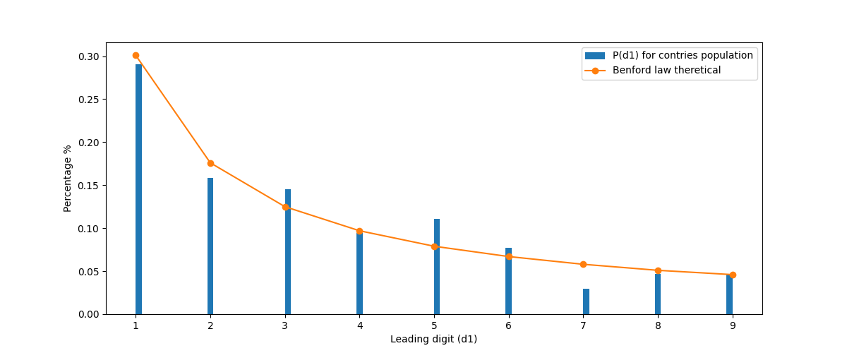
How can this happen? Well, Benford’s Law. (Re)Introduced by the physicist Frank Benford, it states that - “… in many real-life sets of numerical data, the leading digit is likely to be small.” In this blog post I will try to justify it why that happens, and what are some use cases of this empirical law.
\[P(D_1 = d_1) = log_{10}(1 + \frac{1}{d_1})\] \[∀d_1 ∈ \{1,2,3,…,9\}\]Which means that the probability that the leading digit 1 is \(P(d_1 = 1) = 30.1\%\), and for 2 is \(P(d_1 = 2) = 17.61\%\) … up to \(P(d_1 = 9) = 4.58\%\). This seems odd. Because it implies that given a real-world dataset like - population of countries, area of countries, world tallest structures, numbers that appear in the financial times, volume of trading in any stock exchange, video lengths in youtube, etc. - we can expect the leading number to be 1, a third of the time. And the strangest thing is that it does not depend on unit, that is to say that if we take the world tallest structures in meters, or feet, they will both conform to Benford’s law leading digit frequency.
Warning: There is a caveat to applying this law. To apply Benford’s law you should keep in mind that the dataset you have at hand has a good deal of range, spanning several orders of magnitude. A rule of thumb would be 3-4 orders of magnitude from the minimum to maximum value should be more than enough. That is not an issue in most datasets, except for specific datasets like adult human height which spans from 1.3 - 2.3 meters approx.
The intuition behind it
In my personal experience, I found it surprising that when considering numbers from 1 to 1000, the distribution of leading digits follows a specific pattern. Specifically, we observe that there are exactly 1 + 10 + 100 = 111 numbers for each leading digit (1 to 9). This pattern, where the count of numbers for each leading digit follows a power of 10, intrigued me. Why would this distribution occur then? To understand why this distribution occurs, we need to simulate and explore further.
First let me generate a bunch of numbers in python and see how the probability of having a specific leading digit changes over time.
1
2
3
4
5
6
7
8
9
10
11
12
13
14
15
16
17
18
19
def get_leading_digit_numpy(numbers):
    dividers = 10 ** np.log10(numbers).astype(int)

    leading_digits = numbers // dividers
    return leading_digits

interested_digit = 1
power = 5
range_ = (1, interested_digit * 10**power + 9 * 10**(power-1) + 10**(power-1))
x = np.arange(*range_)
logx = np.log10(x)
leading_digit = get_leading_digit_numpy(x)

cumulative_sum = np.cumsum(leading_digit == interested_digit)
indices = np.arange(1, len(leading_digit) + 1)
dist = cumulative_sum / indices

mean_dist_val = np.mean(dist)
mean_dist = np.cumsum(dist) / indices
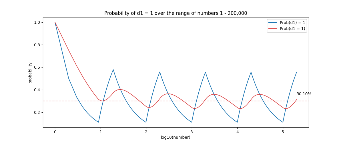
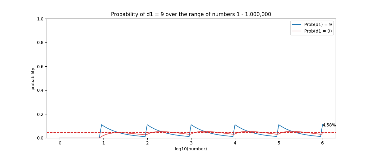
Figure 2 shows a sawtooth pattern of the probability of a digit occurring (\(d_1 = 1\) in our case). That means that from 1-2 we have a 50% chance of having a leading digit 1, then 1-9 it goes down to 1/9 = 11%, however, when in the next 10 numbers 10-19, the probability of having a 1 goes up to 57%. It decreases again up to 99, then it increases for the next 100 numbers. This patterns forms our sawtooth, and tracking the mean of it (red line), we can sense it approaches some specific value towards infinity.
Another way that plays a major role into this distribution is the relative difference between numbers. Say that we have the number 100, if we want to increase it to 200, we say that we have increased it by 100%. Let’s then see about 900, if we want to increase it by the same absolute value, we get to 1000, but that is a mere 10% increase. What this implies is that a number that is in the range of 900, is far easier to jump into the range of 1000, and by the same token the frequency of the leading digit moves from 9 to 1, making 1 more probable. Whereas in the other hand, having a value equal to 100, we have to have a 100% increase to change the leading digit.
Not just the leading digit, Benford’s law can be applied further to the first two leading digits. This is a bit more specific and involved, but the intuition is very similar as with the leading digit.
\[P(D_1D_2 = d_1d_2) = log_{10}(1 + \frac{1}{d_1d_2})\] \[∀d_1d_2 ∈ \{10,11,…,99\}\]Applications
Having a formula on how distributions of a large array of datasets should look like, is a very powerful tool to have on your tool belt. One very practical use case of Benford’s law is in accounting. More specifically, forensic accounting, that is to discover unlawful behaviour in shady businesses. In fact fraud detection based on Benford’s law should be one of the first tests to do when you do not know where to start. It is simple and might help you to focus on the digits that do not “behave” to the pattern.
To test the goodness of fit for Benford’s law we can use a variety of metrics, such as MAD (mean absolute deviation), formally stated as such:
\[MAD = \frac{\sum_{i=1}^{K} |E_i - A_i|}{K}\]where K is the number of bins (9 in the one digit Benford’s test), \(E_i\) is the expected theoretical distribution for that digit, and \(A_i\) is the actual distribution found. The lower MAD value is, the better the fit (or conformity to Benford’s Law).