Blue noise is an interesting concept used in so many generative art and science. From the distribution of light capturing cones in your eye, to modern 3D printers, and many more. In practical terms blue noise referees to a random field of points, where there is not any “visible” clustering of points. This is a somewhat relaxed interpretation of the concept of “point cloud without visible clustering.” Nevertheless, it remains an interesting and valuable property.
Why so blue?
When I think about blue noise, I cannot stop but think of Chet Baker - Almost Blue. It is captivating, bluesy, and it makes me feels distant. That is why today I am going to explore this topic and dive into how we can generate this type of noise. I will not be showing any code as there are a lot of more proper ways of generating it, and the main goal of this post is to give you an understanding rather than creating “trve blue noise.”
Definitions
I think it is better to show the difference between white vs blue noise by a example rather than diving into technicalities (see figure 1).
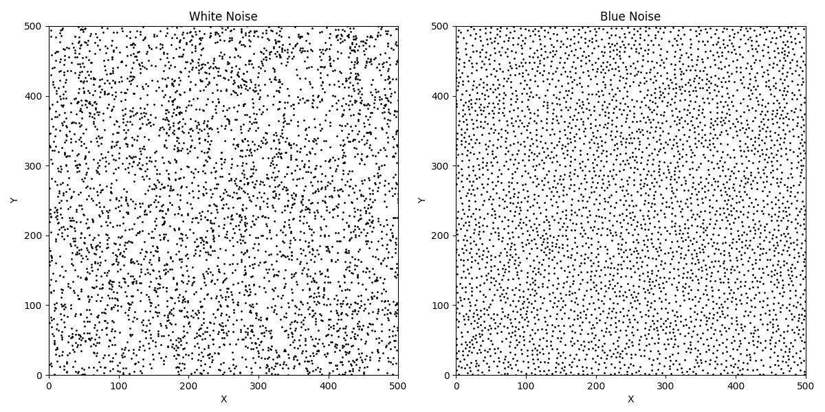
Even though both of these 2D points are generated randomly, the one on the right feels a bit more distant, thus the term blue. In the case of white noise we can see some clusters of points in several places. In contrast, the blue noise plot doesn’t immediately see any clusters forming.
Feels like blue
Before explaining how we can generate them, we need to understand what are the inputs of a blue noise generator. First would be the dimensions of the canvas, width x height, then we would want to specify the spacing radius. The latter is used to determine that no two points should be less than this spacing radius. That is one of the properties that if we can respect, we will generate “almost” blue noise. This is not the only condition as its important to fill the canvas uniformly as well.
Almost blue
There is a not so well known function inside scipy.ndimage called distance_transform_edt. This function is crucial into abiding by the first
constraint, “no two points should be closer than the spacing radius.”
The animation you are seeing is coming from the call distance_transform_edt(1 - img), which basically gives a density of which coordinate
is the furthers from the image, which is a binary image of where there are (x, y) points on the canvas. After computing this density by the
following script you can sample from this distribution such that - areas that are brighter have a higher chance of being picked than darker areas.
1
2
3
4
5
6
7
8
9
def generate_new_random_point(density, index_arr, n_points):
    initial_prob = density.reshape(-1)
    initial_prob = np.divide(initial_prob, np.sum(initial_prob))

    idx = np.random.choice(index_arr, size=n_points, p=initial_prob)
    idx = np.unravel_index(idx, density.shape)
    idx = np.stack([idx[1], idx[0]]).T

    return idx
This is a trick to get the next random point to abide by the rule about the spacing radius. However, this does not ensure 100% that we get correct blue noise (see figure 3).
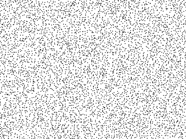
This is close to what we want but not exactly. We need a way to only select the points that have broken the first rule, remove them, and add new points that are much obedient.
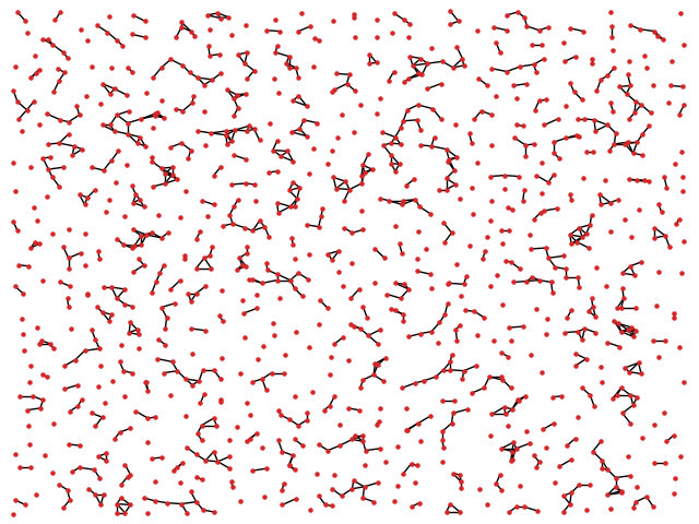
Using some numpy matrix manipulation and the library networkx we can find every node that breaks the rule and connect them together
(see figure 4). Now from this point we iterate over each connected component, and find the middle point. We remove the connected component and add in the new point. This method however is not perfect, and may sometimes fail due to something called convex hull of the points. When we find the mean/middle of the points, we are implicitly creating a convex hull of all points and we are finding the middle of that shape. However, if that shape is mostly concentrated on the edges it might be the case that the new point we introduce will break the rule we have for the spacing. However, in practice this is not that visible.
Conclusion
In this post we saw the basics of what is blue noise, and how can we conceptually create it. Even though I did not provide code, I will update this post to link to my github whenever I clean up the script to generate blue noise. I felt showing the full code to generate blue noise would have been a bit cumbersome, rather I opted for some snippets to show the general algorithm how it might work.