A large part of our time as Data Scientist revolves around exploring and familiarizing ourselves with different datasets. And a huge portion of these datasets are by nature, multi-dimensional.
We are not in luck if we have more than 3 dimensions as the data is difficult to visualize. We resort to either pair plotting, or some fancy method of dimensionality reduction techniques. One common example is getting to know the distribution of a dataset by plotting its histogram. This is very easy in 1-D and 2-D case. 3-D becomes tricky but still manageable. After that we get lost. We can use tricks like color and size as another dimension, but doesn’t mean that anybody but us will understand us.
A resolution to this problem are what is known as parallel coordinates. These are very easy conceptually as we do not have orthogonal lines crossing each other, but rather multiple parallel lines some fixed distance from each other. They are easy to visualize, however how does a histogram can be visualized in this coordinate system? We will build our intuition behind this during this article.
Imports
1
2
3
import numpy as np
import pandas as pd
import matplotlib.pyplot as plt
Dimension one: tying our shoes
We need to start with the basics of histograms, and their usages before jumping in more detail. Necessary first step is plotting a basic histogram.
1
2
x = np.random.normal(0, 1, 10000)
plt.hist(x, bins=100);
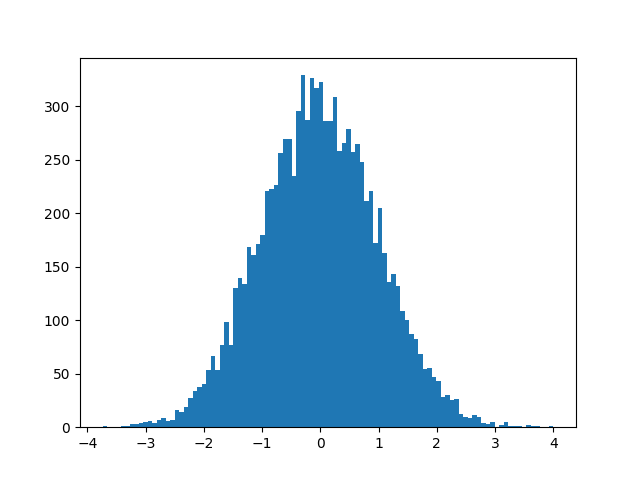
Simple, and concise. What the histogram represents is if we were to ask the data a lot of times “how many points are between a and b for each x (formally: \(a \le x_i \le b\))?”.
Dimension two: one up
Now that we know the 1-D case, how about 2-D…
1
2
3
4
5
mean = [0, 0]
cov = [[1, 0], [0, 1]]
x, y = np.random.multivariate_normal(mean, cov, 10000).T
h, xedges, yedges = np.histogram2d(x, y, bins=50)
plt.imshow(h, cmap='inferno')
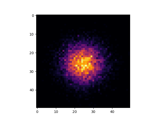
We are doing the same thing here, just the computation of the histogram comes from numpy rather than matplotlib, which calls numpy under the hood.
np.histogram2d from numpy computes for each “pixel” the count that it saw for that “pixel”. Now instead of using pixel, we use the term bucket.
We are splitting the data into buckets and measuring how much data is in each bucket.
From this function we also get edges (up and down) which are the intervals \(A \le x_i \le B\) or \((a_1, a_2) \le (x_{i,1}, x_{i,2}) \le (b_1, b_2)\). These 4 points A and B define the rectangle that defines a bucket. And our data point \((x_{i,1}, x_{i,2})\) it either is in this bucket or not.
Parallel coordinates
Visualizing 3D data can be trickier since we need to build a volume, or a point cloud, which is not very straightforward to understand the structure of your data. So for this reason we will use a different coordinate system.
This is better shown with the following example:
1
2
3
4
5
6
7
8
9
10
11
12
13
14
15
16
17
18
19
20
21
22
23
24
x = [1, 5, 6, 7, 3, 4]
y = [2, 1, 6, 10, 5, 1]
fig, (ax1, ax2) = plt.subplots(1, 2, sharey=True, figsize=(15,7))

ax1.plot(x, y, 'ro')
ax1.set_xlabel('X1')
ax1.set_ylabel('X2')
for x1, x2 in zip(x,y):
    ax2.plot([1, 2], [x1, x2] , 'ro')
    ax2.annotate("", xy=(2, x2), xytext=(1, x1),
            arrowprops=dict(arrowstyle="->"))

    ax2.annotate("", xy=(1, x1), xytext=(x1, x2),
                 xycoords=ax2.transData,
                 textcoords=ax1.transData,
                 arrowprops=dict(arrowstyle="->", linestyle='--', alpha=0.15)
                )

    ax2.text(1, x1 + 0.2, f"{x1}")
    ax2.text(2, x2 + 0.2, f"{x2}")
    ax1.text(x1 - 0.2, x2 + 0.15, f"({x1}, {x2})")
ax2.set_xlim((0.9, 2.1))
ax2.set_xticks([1, 2])
ax2.set_ylabel('X1, X2');
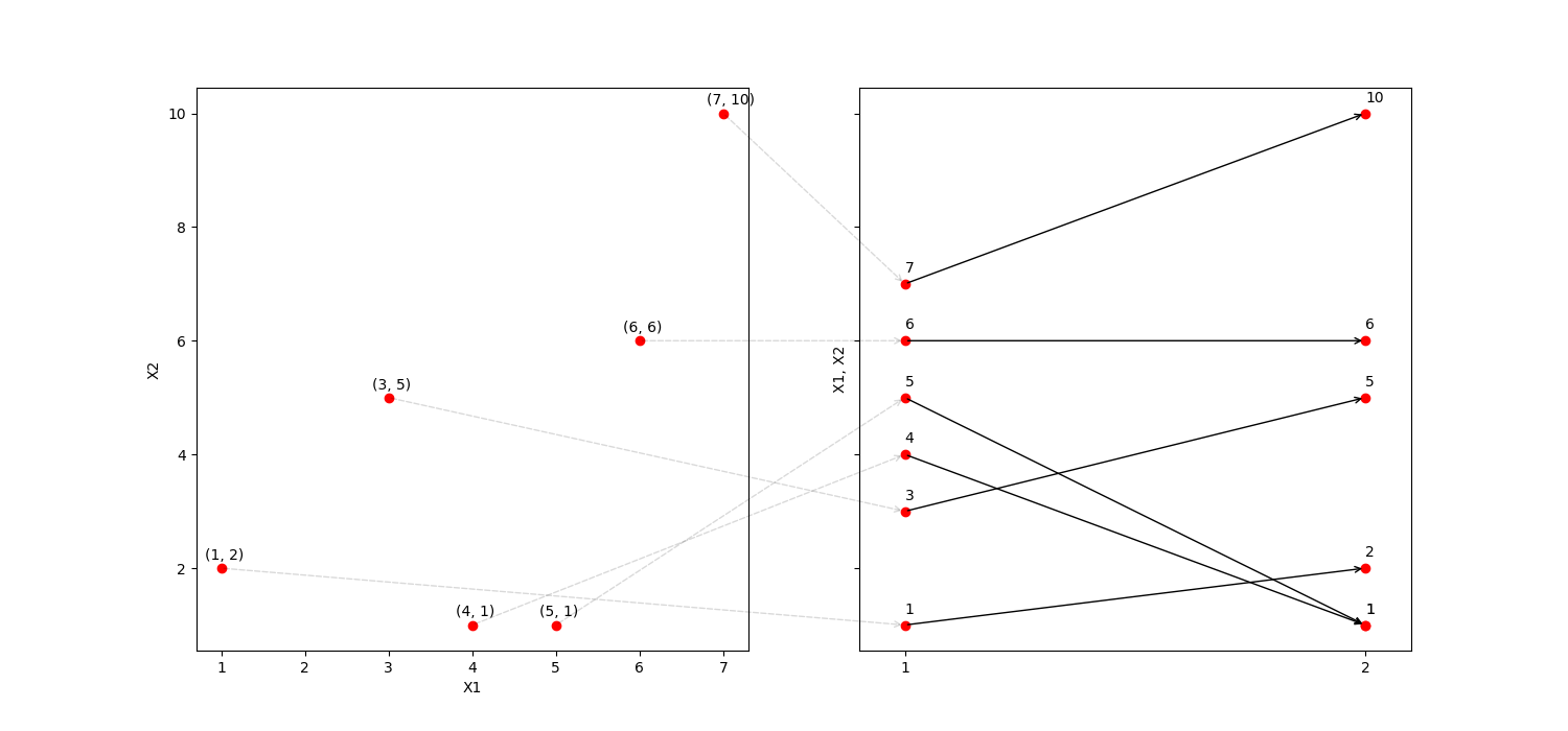
Here we can see on one side the 2-D coordinate system, and its translation to parallel coordinate system. If we would have a 10-D point, we would represent it with 10 points in the parallel coordinate system.
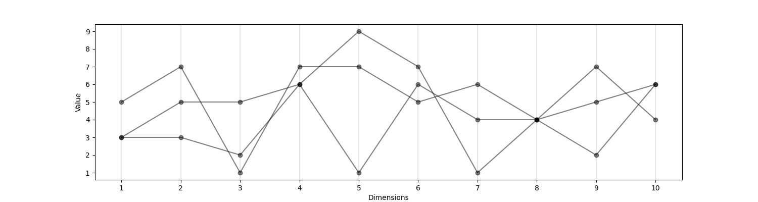
Nice, we got this one covered. Next we will discuss the tricky part what does it mean to take the histogram in this coordinate system. In the next post we will take a look at this system, some use cases and connection to Gaussian Processes.